Mathematician Katherine Johnson is famous for calculating trajectories of America's first manned space missions for Project Mercury as depicted in the movie Hidden Figures.
The big concern at that point in the history of the space program was accurately predicting where a spacecraft would land in the ocean after re-entering the earth's atmosphere. Any miscalculation could send the mercury capsule hundreds of miles from where the Navy was expecting to recover the spacecraft and the astronaut inside.
The calculation that Katherine Johnson did had to consider many different effects on the trajectory of the mercury capsule. In an earlier activity we considered how fast the mercury capsule needed to be moving to make multiple orbits of the earth (which was one of the main goals of Project Mercury).
In this activity we will consider how the mercury capsule comes back to earth. This part of the space mission is referred to as "re-entry". Eventually your program will look like this:
Step 0. Check out this modified version of the program from the end of Project Mercury (Part 1. Circular Orbit)
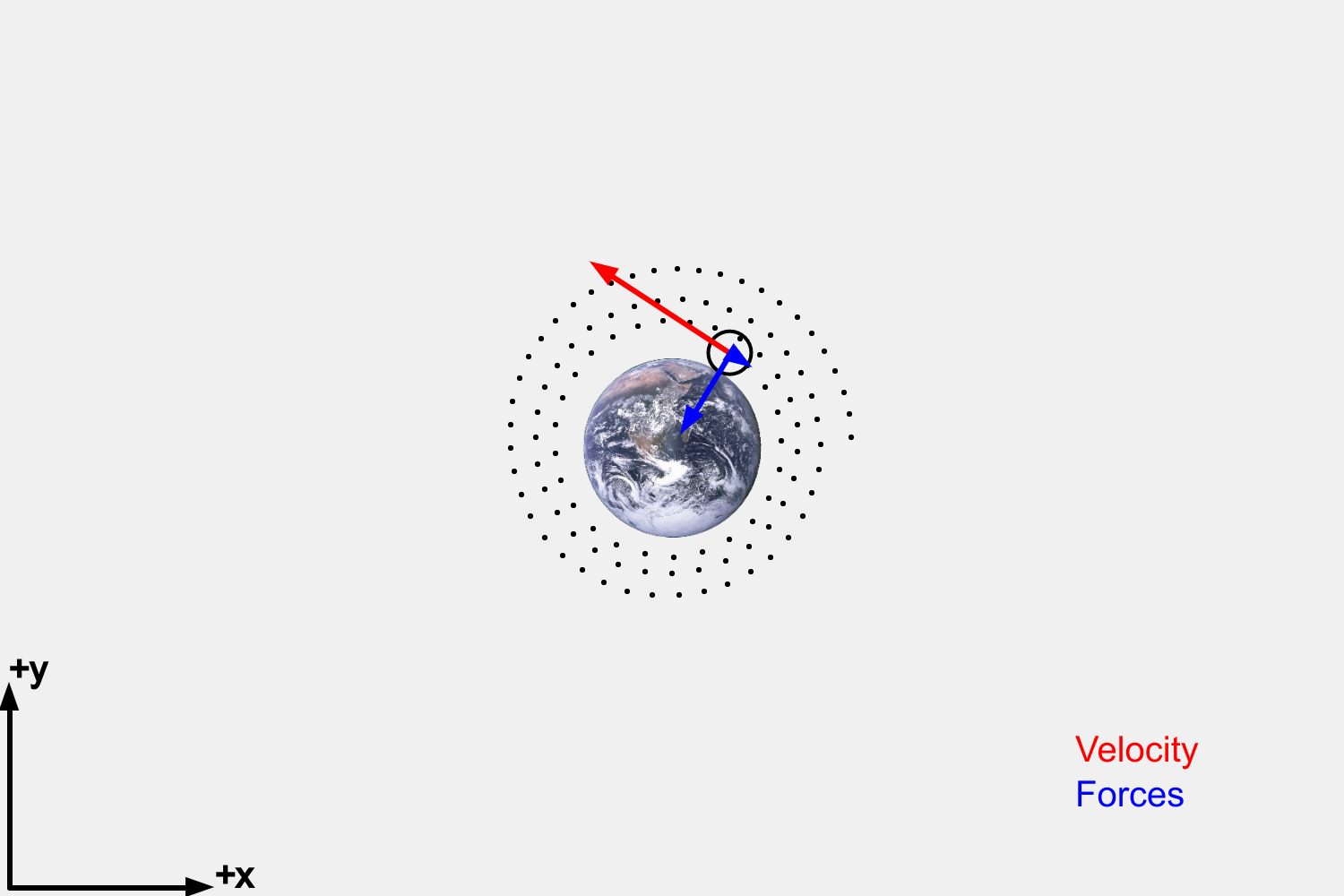
Step 1. Note the velocity and initial position
Notice that the initial velocity and position have changed from the earlier Project Mercury activity.
// Initial velocity of the Mercury capsule
vx = 0;
vy = 31.63;

// Initial position of the Mercury capsule
x = 475;
y = 250;
The initial velocity is a bit slower than what we used at the end of the earlier activity and the initial position is a bit further from the earth than in the earlier activity. This is partly to not give away the answer to the earlier activity and partly so we can see the Mercury capsule orbit the earth a little bit better.
Step 2. Count the number of orbits
The goal of Project Mercury is for the capsule to make a few orbits of the earth and then to splash down into the ocean. Let's add some code to count the number of orbits.
At the beginning of the code add a variable to keep track of the number of orbits so far
orbits_so_far = 0;
Inside the draw function but after the display() function add some code to detect each time the capsule returns to it's initial y position with a positive velocity in the y direction
    // if the position of the capsule is near y = y_earth
    if ((abs(y - y_earth) < 0.5*abs(vy)*dt) & vy > 0) {
        orbits_so_far += 1;
    }
    drawText('orbits so far = ' + orbits_so_far,0.05*width,0.9*height);
After you add this to your code your program will behave like this
Step 3. Add air resistance to the simulation
Have you ever put your hand out the window in the car and noticed the force of the air on your hand as the car is moving? The same thing happens when you are moving thousands of miles an hour! And it happens in space even though the density of the air up there is a fraction of what it is on the ground.
The force you experience when you travel quickly through the earth's atmosphere is called air drag (a.k.a. air resistance). The code you are working with now does not include air drag, but we can add that now.
Here is the part of the code we are going to modify:
  Fx = -Fgrav*cos(theta);
  Fy = -Fgrav*sin(theta);
We need to add air drag to this code. The force produced by air drag is given by this equation: $$ F_D = \frac{1}{2} \rho A C_D v^2 $$
where $A$ is the cross sectional area of the object, $\rho$ is the density of the air, $C_d$ is the drag coefficient and $v$ is the speed.
The drag coefficient $C_d$ is a unitless number that has to do with how pointy or how flat the object moving through the air is. Flatter objects have more air resistance, so the drag coefficient is larger. A typical drag coefficient for a flat object is 1.0 which is what we will assume here. Pointy objects have a drag coefficient closer to 0.1 but the Mercury capsule reenters the big round end goes first so it is more like a flat object than a pointy object, so we will use $C_d \approx 1.0$.
The code below implements the equation for $F_D$ into the code as another force in addition to gravity. The extra minus sign is because the drag force is in the opposite direction of the motion.
    Cd = 1.0;  // drag coefficient
    rho = 1.0; // density of the air
    A = 0.001; // area of the capsule

    Fdragx = - 0.5*rho*A*Cd*sqrt(vx*vx+vy*vy)*vx;
    Fdragy = - 0.5*rho*A*Cd*sqrt(vx*vx+vy*vy)*vy;

    Fx = Fgravx + Fdragx;
    Fy = Fgravy + Fdragy;
After you implement this into your code you will notice that the Mercury capsule comes down to earth after making a few orbits. How many full orbits does it make before it lands?
Optional: Just for fun, visualize the drag force by changing this:
drawBlob(x,y,vx,vy,Fgravx,Fgravy,0,0);
to this:
drawBlob(x,y,vx,vy,Fgravx,Fgravy,Fdragx,Fdragx);
After you add all these things to your code your program will behave like this
The last orbit is really important because it is the one where the capsule lands in the ocean. We have been counting the orbits but we need to figure out how much of the last orbit that the Mercury capsule completes. Is it 10% of the last orbit? 90%? Something in-between? The exact number determines where the Mercury capsule will land!
We can use the angle that the capsule makes with the center of the earth to figure out how much of the final orbit is completed. This angle is a little bit like the longitude where the craft will land.
Good news: The code already measures the angle! Here is the line of code that measures the angle:
theta = atan2(y - y_earth,x - x_earth);
This is taking the arctangent of the right triangle that the capsule makes with the center of the earth where the hypotenuse is the distance from the center of the earth to the capsule.
Show the value of theta on screen by adding this code:
    drawText('theta = ',0.05*width,0.85*height);
    drawText(theta,0.15*width,0.85*height);
    drawLine(x_earth,y_earth,x,y);
    drawLine(x_earth,y_earth,x_earth+earth_radius,y_earth);
The drawLine functions there help to highlight the angle that we are measuring.
After you add this code so you can see the value of theta, is the angle in degrees or radians?
Now you can measure the final angle that the mercury capsule makes which is important because you can use this to figure out what fraction of an orbit that the capsule makes on the last orbit. Is it 10%? Is it 90%?
What is the total number of orbits plus this fraction? 4.2? 5.7? 10.9? etc. This is an important number because the team charged with picking up the Mercury capsule can use that number to figure out exactly where the landing will be.
What is the total distance traveled by the Mercury capsule? Use the number of orbits plus the fraction you calculated to figure it out. Remember that earth_radius = 50;
Hint: For each orbit the Mercury capsule moves one circumference.
Step 6a. Theory
The task for Katherine Johnson was to double check the result of the simulation. Computer simulations can fool us! Errors can happen. Astronaut lives hang in the balance.
In the last activity we used $F = ma$ to double check the result of the simulation. For this activity we can use energy conservation and the fact that the orbit is losing energy due to the drag force. The basic idea is that this is a complicated simulation but if you add the initial kinetic energy an the initial gravitational potential energy, then at a later time, the remaining kinetic energy plus the remaining potential energy plus the energy lost due to air drag should add up to the same number. Mathematically this relationship can be written: $$ KE_i + PE_i = KE_f + PE_f + E_{\rm loss} = {\rm constant} $$
The kinetic energy $ KE_i = (1/2) m v_i^2 $ and the remaining kinetic energy is $ KE_f = (1/2) m v_f^2 $. The initial gravitational potential energy is $PE_i = - G M m / r_i $ and the remaining gravitational potential energy is $PE_f = G M m / r_f $. As in the earlier exercise, $G$ is Newton's gravitational constant, $M$ is the mass of the earth and $m$ is the mass of the Mercury capsule.
Step 6b. The Energy Loss term
Let's talk about the energy loss term. In introductory physics one of the equations that you learn is this one: $$ {\rm Work} = {\rm Force} \cdot {\rm distance} $$
And "work" is just another word for energy.
For the energy lost to air drag the force here is clearly $F_D$ from earlier. The distance is the distance traveled in the orbit. $$ E_{\rm loss} = F_D \cdot d = \frac{1}{2} \rho A C_D v^2 d $$
In principle, the density could be changing with time because the density changes with height above the earth's surface, but for now at least we are just going to keep the density constant.
An important question is what to use for $v$ in the equation above. Do we use the initial speed ($v_i$)? Or the final speed ($v_f$)? Because the drag force is acting on the entire trajectory the best answer turns out to be the average of the initial and final speeds. Our equation for $E_{\rm loss}$ becomes $$ E_{\rm loss} = \frac{1}{2} \rho A C_D \left( \frac{v_i + v_f}{2} \right)^2 d = \frac{1}{8} \rho A C_D \left( v_i + v_f \right)^2 d $$
Step 6c. Assume a circular orbit
If you watch the simulation, as the Mercury capsule comes down to earth the orbit stays very close to circular even as the distance between the capsule and the earth decreases.
In the first part of this activity we concluded that anything moving in a circular orbit due to gravity should have a speed given by this equation: $$ v = \sqrt{\frac{G M }{r}} $$
We can use this to rewrite $KE_i$ and $KE_f$ in our expression $$ KE_i = \frac{1}{2} m v_i^2 = \frac{1}{2} m \left( \sqrt{ \frac{G M }{r_i}} \right)^2 = \frac{G M m}{2 r_i}$$
We can do the same thing with $KE_f$ $$ KE_f = \frac{1}{2} m v_f^2 = \frac{1}{2} m \left( \sqrt{ \frac{G M }{r_f}} \right)^2 = \frac{G M m}{2 r_f}$$
Step 6d. Simplify the expression
As a reminder we are using this expression to model the orbit: $$ KE_i + PE_i = KE_f + PE_f + E_{\rm loss} = {\rm constant} $$
Using what we know now we can re-write this expression like this: $$ \frac{GM m }{2 r_i} - \frac{G M m }{r_i} = \frac{G M m}{2 r_f} - \frac{G M m }{r_f} + \frac{1}{8} \rho A C_d \left(\sqrt{\frac{G M}{r_i}} +\sqrt{ \frac{G M }{r_f}} \right)^2 d $$
This expression can be simplified to this expression: $$ - \frac{GM m }{2 r_i} = -\frac{G M m}{2 r_f} + \frac{1}{8} \rho A C_d \left(\sqrt{\frac{G M}{r_i}} +\sqrt{ \frac{G M }{r_f}} \right)^2 d $$
Step 6e. Solve for d
Use the values from the program to solve for $d$. Look at the program to get the valuese for $G$, $M$, $m$, $\rho$, $A$, $C_D$, $r_i$ and $r_f$
Note that you can infer $r_i$ and $r_f$ in the code from the initial $x$, $y$ position of the mercury capsule, the center of the earth ($x_{\rm earth}$, $y_{\rm earth}$) and the radius of the earth ($r_{\rm earth}$).
After you solve for $d$ divide it by the circumference of the orbit to figure out how many orbits the object will make. $$ {\rm orbits} = \frac{\rm distance}{\rm circumference} = \frac{d}{2 \pi r} $$
Note: Because the orbit is shrinking (starting with $r= r_i$ and ending with $r = r_f$) use the average radius to calculate the circumference by averaging $r_i$ and $r_f$.
Challenge: Don't use a calculator to do any of the calculations!!! See if you can do it by hand like Katherine Johnson did!
In Step 5 we measured the number of orbits from the program. In Step 6 we used energy conservation to estimate from theory how many orbits should happen before the Mercury capsule lands. One of the things Katherine Johnson had to do was to compare the prediction by the computer simulation to her prediction from the mathematics.
A typical way to measure the percent error is this formula: $$ \% = 100 \cdot \frac{|\rm measured - true|}{\rm true} $$
Use this formula to compare the number orbits. To do this you will need to decide whether to treat the math as "true" and the computer simulation as "measured" or the computer simulation as "true" and the math as "measured". (It depends on whether you think the math or the computer simulation is more accurate -- or maybe you can think of a way of obtaining the percent error by assuming that they are both equally accurate...)
Challenge: Calculate the percent error without using a calculator! Do it by hand like Katherine Johnson did!
In what we have done so far we have compared the number of orbits in the computer simulation to the number of orbits predicted from energy conservation. As you saw in Step 7, these two numbers don't agree perfectly.
Even though it seems very reasonable, it turns out that this equation that we used is not as accurate as it could be: $$ {\rm orbits} = \frac{\rm distance}{ \rm circumference} = \frac{d}{2 \pi (\frac{r_i + r_f}{2})} $$
The problem with this equation is that the Mercury capusule does more orbits closer to the Earth ($r = r_f$) than it does further away ($r = r_i$). A better rway to compare theory and the computer simulation is to measure the distance traveled in the computer simulation.
Here is some code you can add after the display() function to measure the distance traveled:
    total_distance = 0.0;
    for (i = 0; i < xhistory.length-1; i++) {
       total_distance += sqrt((xhistory[i+1] - xhistory[i])**2 + (yhistory[i+1] - yhistory[i])**2);
    }
    drawText('total distance = ',0.4*width,0.8*height);
    drawText(total_distance,0.65*width,0.8*height);
After you add this code, you can compare the number that you get for the total distance to $d$ which you obtained in Step 6. Go ahead and calculate the percent error (as described in Step 7). The percent error should be smaller than what you originally got in Step 7 when you were comparing the number of orbits, even though the simulation is exactly the same as before and even though $d$ is the same as it was earlier. Comparing the distance traveled turns out to be the best way to compare the theory to the computer simulation.