V.B.4.e.3.ii. Ethyl cyanide
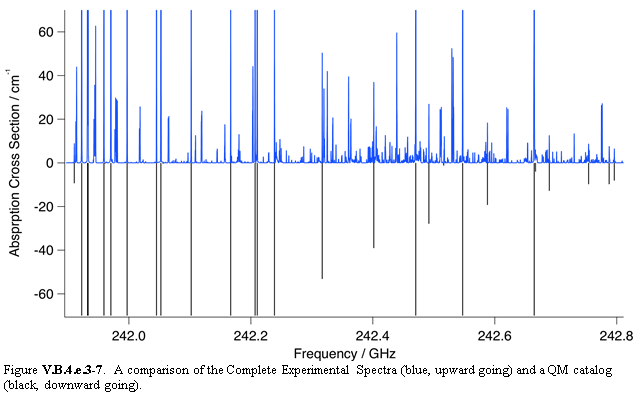
Next we consider ethyl cyanide to illustrate the impact of a more complex spectrum with many uncataloged lines, a more complicated lineshape, and optical thickness. Ethyl cyanide has a considerably denser and more complex spectrum than methyl cyanide. Figure V.B.4.e.3-7 shows a stick spectrum comparison of the QM simulation of the ethyl cyanide spectrum with one based on the CES. It should first be noted for lines that are in both the QM catalog and the CES the intensities are in good agreement. This is a required byproduct of using the QM intensities to calibrate the intensities in our experimental spectra and the accuracy of the experimental intensity calibration. More importantly, this figure shows the many uncataloged lines that contribute both to new features in the ALMA spectra, and shoulders and additional intensity where there is overlap. This can be seen in more detail in Fig. V.B.4.e.3-9 where we combine the CES and astrophysical lineshapes to simulate the ALMA spectrum in this region.
We have chosen the region near 224 GHz shown in Fig. V.B.4.e.3-8 to determine the intensities and optical thickness of ethyl cyanide. In this figure the ALMA spectrum is shown in black, in blue is the simulation (including effects of optical depth), and in dashed red is the simulation without the effects of optical depth. It is clear that optical thickness plays a major role in the ALMA spectrum of ethyl cyanide.
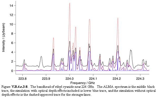
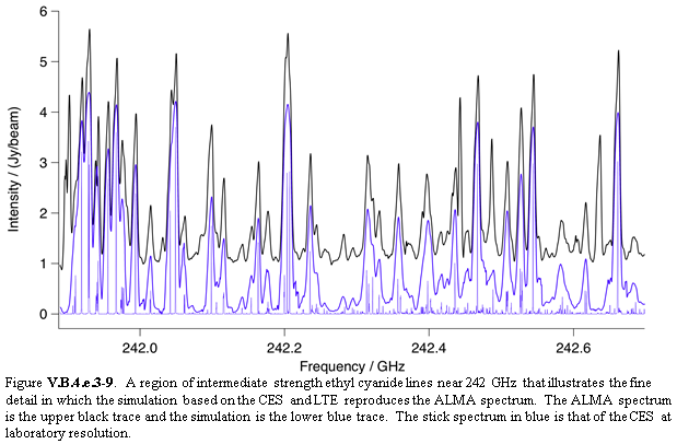
When lineshape and optical thickness effects are convolved with the 190 K simulation from the CES of Fig. V.B.4.e.3-8, the result is Fig. V.B.4.e.3-9. Not only does the completeness of the CES result in the simulation of many new features, but it also accounts for many subtle lineshape effects. It is also significant that the intensity scaling factor and optical depth that were determined by the intensity fit near the bandhead in Fig. V.B.4.e.3-8, were applied in Fig. V.B.4.e.3-9 without further adjustment. Given the very substantial contributions of the uncataloged lines to the good agreement in Fig. V.B.4.e.3-9, this shows the importance of these contributions to showing the simple LTE model used here accounts for a wide range of rotational and vibrational states.
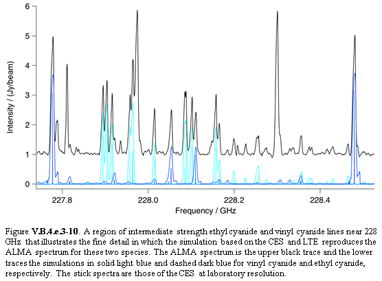
Figure V.B.4.e.3-10 provides additional detail. The top trace (blue) is the difference between the ALMA spectrum and the CES and the second trace from the top (red) is the difference between the ALMA spectrum and a simulation based on the QM catalog. Positive difference can be attributed to lines other than those of the ethyl cyanide simulation. For a more direct comparison, below the ALMA spectrum are the simulations based on the QM catalog (red - dashed) and the CES simulation (blue). While the CES simulation is very good, we expect that when we do a more careful adjustment of intensities and lineshapes in a global fit that additional reductions in the residuals will occur, especially in the regions that include optically thick lines.