V.C.3 Typical Results of the Core Spectrometer
The great strength of SMM rotational spectroscopy is its specificity, especially when applied to complex mixtures. A recent paper considered the clutter issue for both the clean and polluted atmosphere in detail and concluded that even in the polluted atmosphere the clutter limit is below 1 ppt [2]. Spectroscopic sensors are typically demonstrated on small mixtures of highly favorable spectroscopic gases such as H2O, NH3, CO, NO, H2O2, HBr, HCl, H2S, etc. For the work described here a much larger mixture, 32 gases, which also include many species with significantly weaker and more crowded spectra was used. While the chosen molecules are generally favorable species for rotational spectroscopy, they range over about two orders of magnitude in both strength and spectral density and contain 17 gases included in a common list of Toxic Industrial Chemicals [3]. Many of these species do not have resolved rotational spectra in the Op/IR and most are considerably less favorable than species typically chosen for demonstrations. Additionally, the near transparency at low pressure in the SMM of H2O and CO2 (molecules that provide significant clutter in Op/IR sensors [4]) makes this approach remarkably clutter free.
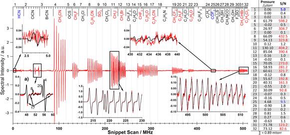
Because the information content in the 210 – 270 GHz region far exceeds that necessary for ‘absolute’ specificity, we chose a subset of six lines for each gas and observed a 2–6 MHz ‘snippet’ for each line—a total of 192 snippets and ~0.5 GHz of spectral space. These results are shown in Fig. V.C.3-1. The snippets are recorded in order of the analyte in the library, to facilitate visual identification of detected gases. Automated analyses, based on least squares techniques (LSQ) and shown in the right panel of Fig. V.C.3-1, provide quantitative results by comparison of the spectra shown in Fig. V.C.3-1 with previously recorded libraries. These LSQ analyses require much less than 1 s. Each of the 14 gases placed in the mixture is identified in red in Fig. V.C.3-1. Those identified in blue are marginal detections that result either from contamination or chemical reactions among the analytes.
Figure V.C.3-1. Observed spectra at each of the six fingerprint regions selected for each gas for the family of 32 gases considered, with blow-ups of specific fingerprint regions. Panel on right shows the results of a quantitative LSQ analysis. A digital lock-in recovers a near first derivative lineshape that results from a small FM modulation on the probe driver.
Insert a of Fig. V.C.3-1 shows a blow-up of the ClCN fingerprint region. No ClCN is present in this mixture, and the signal in this region is from the interloping spectra of other species, CH3CN, C2H3CN, C2H5CN, and C2H3F. However, because of the intensity calibration of the system, the fit for the concentration of these four species fully accounts for these spectral features. Accordingly, the fit properly concludes that although there is spectral intensity in the ClCN fingerprint, less than 0.01 mTorr of ClCN is present. The partial pressures of each gas recovered by the LSQ fit ranged from 0.02–0.13 mTorr. The total pressure measured spectroscopically was 0.89 mTorr. This pressure is within the accuracy of the pressure measurement of the fill of the sample cell, nominally 1 mTorr.
Operation at this low pressure (and correspondingly low probe power) provides for accurate intensity calibration and signal recovery with known lineshapes, even in complex mixtures. This allowed the accurate overlap subtraction shown in Fig. V.C.3-1. If this system were instead optimized for sensitivity (which is possible in software) increasing the pressure until the pressure broadening equals the Doppler Broadening (around 10 mTorr) would provide increased fractional absorption and allow probe powers that scale with the square of the sample pressure.
Because the pressure is low, all of the lines have widths determined by Doppler broadening. Thus the species are spectroscopically non-interacting and it is possible to determine their minimum detectable concentration individually. If we first consider the strongest species in this figure, CH3CN, a sample pressure of 6 x 10⁻⁵ Torr produces a S/N of ~500 with 0.01 s per point of integration time. Each of the 6 lines has ~10 points. If each point receives 1 s of integration time and a fit is used to process all of the information in the ~60 points on the lines, the S/N for this recovery becomes ~ 40,000. Thus, for a 1/1 S/N on the recovery a pressure of ~1.5 x 10⁻⁹ Torr would be required. To obtain a ppx measure, the fact that an air pressure of ~0.1 Torr can be added without significantly broadening or decreasing the line, provides a detectivity level of 15 ppb. Figure 3 also shows that the weakest of the 32 gases (C2H4Cl2) is about 30 times weaker, resulting in a detection level of ~500 ppb. The most favorable gas, HCN, is about 5 times stronger, resulting in a detection level of ~ 3 ppb. Similar results have been obtained more directly on samples diluted in air.
Even with this system, which is optimized for specificity and intensity calibration rather than sensitivity, a comparison of the results presented here with those obtained in a wide variety of Op/IR experiments show that they are similar in terms of ppx sensitivity, with wide variation according to choice of molecule and the trades of technical implementations [3, 5-8]. Because the optimum pressure (which is proportional to the Doppler width and thus to frequency as well) is 100 – 1000 times smaller in the SMM, in terms of the minimum sample required, the SMM is correspondingly more favorable according to this measure: ~10-14 moles for HCN, ~ 5 x 10-14 moles for CH3CN, and 10-12 moles for C2H4Cl2. For radicals, for which a strong electronic transition is available, detection limits in the ppt range have been reported [9].
Finally, there is a clear path to even simpler and cheaper systems in the near to medium term. Inexpensive technology is commercially available up to 100 GHz courtesy of the wireless communications industry, and this upper frequency limit is increasing rapidly. While we used instrumentation synthesizers, etc., implementations based on chip level integrations of these functions are available. Finally, the never-ending increase in computational power will further improve our ability to optimize the use of the information content of high-resolution rotational spectra. This combination of analysis power and practicality will allow SMM rotational spectroscopy to take its place alongside other methods as a general analytical and sensor tool in the near term.
[1] I.R. Medvedev, C.F. Neese, G.M. Plummer, F.C. De Lucia, Opt. Lett., 35 (2010) 1533-1535.
[2] I.R. Medvedev, C.F. Neese, G.M. Plummer, F.C. De Lucia, Applied Optics, 50 (2011) 3028-3042.
[3] The Clean Air Act of 1990, (1990).
[4] M.J. Thorpe, D. Balslev-Clausen, M.S. Kirchner, J. Ye, Optics Express, 16 (2008) 2387-2397.
[5] Y. He, B.J. Orr, Appl. Phys. , B 85 (2006) 355-364.
[6] M.J. Thorpe, K.D. Moll, R.J. Jones, B. Safdi, J. Ye, Science, 311 (2006) 1595-1599.
[9] G. Mejean, S. Kassi, D. Romanini, Opt. Lett., 33 (2008) 1231-1233.