Arts College 755
Call No 02463-2
Req: 752
OSC 1224 Kinnear
Fishbowl (rm205)
TR 2-348
Winter 2008
05 credits

Shader Basics

Due date: 01/10, before class.

Section 1: Function Graphing

Graph each of the following functions over the specified domain. Plot x along the x-axis and f(x) along the y-axis. Under each graph, write the range of the function over the specified domain. See the Regular Patterns section of RManNotes for definitions of step, smoothstep, and mod (mod(a, b) returns the remainder of a/b).

1. f(x) = 2
   x domain: [0,1]
2. f(x) = 2 * x - 1
   x domain: [0, 1]
3. f(x) = (x + 1) * 0.5
   x domain: [-1, 1]
4. f(x) = step(0.5, x)
   x domain: [0,1]
5. f(x) = smoothstep(0.4, 0.5, x)
   x domain: [0,1]
6. f(x) = smoothstep(0.1, 0.9, x)
   x domain: [0,1]
7. f(x) = mod(x, 1.0)
   x domain: [0,4]
8. f(x) = mod(x * 4, 1.0)
   x domain: [0,1]
9. f(x) = step(0.5, mod(x * 4, 1.0))
   x domain: [0,1]

Section 2: "One-line" shaders experiments

1. In your favorite text editor create a file called experiment.sl. Put the following text in the file and save it.

   surface experiment()
   {
      Ci = color (1,0,0);
   }
   

2. The above is a complete RenderMan shader. Compile it by using the shader command with the name of the shader text file experiment.sl:

   Z:\> shader experiment.sl
   experiment: compiled.
   

If the shader program prints output other than that above or it prints an error message, double check experiment.sl to make sure it is exactly the same as the text described in step 1.

3. Save the file square.rib in the same folder. Look inside and see that it defines a single patch, with the shader "experiment" applied to it.

4. Render the file by typing, "prman square.rib" on a command line.

   You should see an image of a flat, red square. The object is a simple grid (actually a bilinear patch) with the shader you just compiled, experiment, applied to it.

Experiment Process

For each of the following experiments, do the following:

1. Replace the 3rd line in experiment.sl, which looks like:

   Ci = color (1,0,0);
   

   with each new, specified line;
2. Recompile the experiment shader
3. Re-render the grid
4. Observe the results, investigate and understand what's going on.

Experiments

1. Ci = color "hsv" (0.5, 0.8, 0.3);
2. Ci = s;
3. Ci = t;
4. Ci = color (s, 0, 0);
5. Ci = color (0, t, 0);
6. Ci = color "hsv" (s, 1, 1);
7. Ci = color "hsv" (0, t, 1);
8. Ci = color "hsv" (0, 1, t);
9. Ci = color (s, t, 0);
10. Ci = step(0.5, s);
11. Ci = step(0.2, s);
12. Ci = step(0.5, t);
13. Ci = smoothstep(0.4, 0.6, s);
14. Ci = smoothstep(0.1, 0.9, s);
15. Ci = mod(s, 1.0);
16. Ci = mod(s * 5, 1.0);
17. Ci = step(0.5, mod(s * 5, 1.0));
18. Ci = smoothstep(0.4, 0.6, mod(s * 5, 1.0));
19. Ci = mix(color (1,0,0), color (0,0,1), s);
20. Ci = mix(color (1,0,0), color (0,0,1), smoothstep(0, 1, s));
21. Ci = spline(t, color (1,1,0), color (1,1,0), color (0,1,0), color (0,0,1), color (0,0,1));
22. Ci = step(t, s);
23. Ci = noise(s, t);
24. Ci = noise(s * 10, t * 10);
25. Ci = noise(s * 50, t * 50);
26. Ci = 0.5+0.5*sin(s*2*PI*4);
27. Ci = mix(color(1,0,0), color(0,0,1), smoothstep(0.3-0.5*sin(s*8*PI), 0.7+0.5*sin(s*8*PI), t));

After trying them all and figuring out why each does what it does, choose several and write brief explanations about why they do what they do.

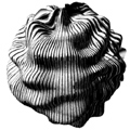
Section 3: make your own!

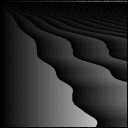
Ci = mod(s,t-.5*t*noise(t*8))

Results:

On your Hw1 web page, show the new one-line shaders you created for Section 3 (both the resulting 256x256 images and the one-line math expressions that generated them.)

(Original version of this assignment by Steve May)

Student Work

Resources:
RManNotes
RMRepository
RenderMan FAQ
Highend3d
Deathfall
Textbook
Pixar
3Delight
Aqsis