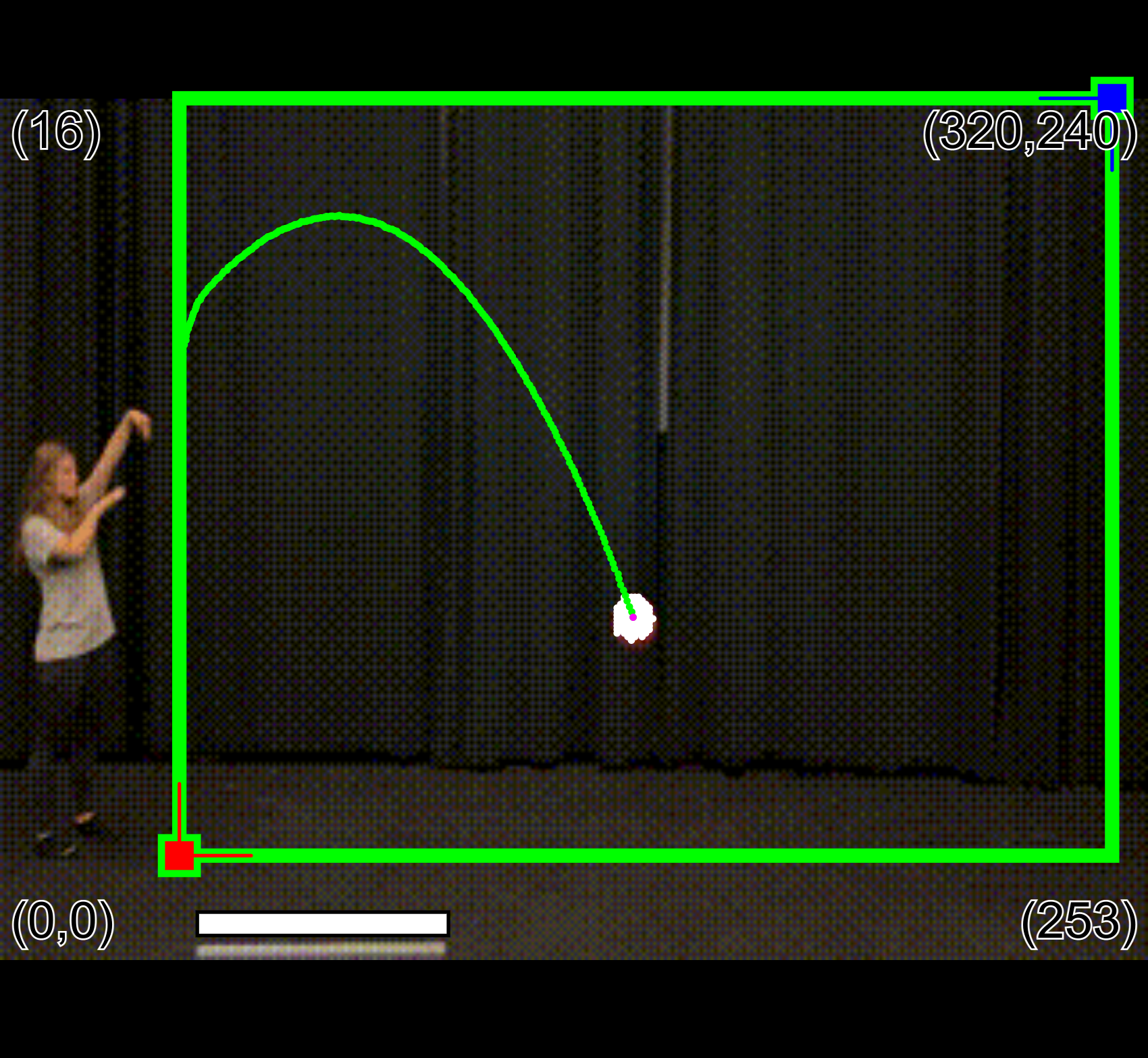
 Step 0. Open the code
Using the data from Part 1 (or Part 2), you will calculate velocities and analyze velocity vs. time plots. You will use these plots to make inferences aboutg and x-acceleration.
 Step 0. Open the code
Click here to open the program
Here are some questions to consider
Find the csv file you downloaded in Part 1 (or your spreadsheet from Part 2) and open it in Excel or Google Sheets.
Add two new columns to the spreadsheet and name them vx and vy. This is where you will calculate velocities.
Recall that the velocity of an object is given by the change in the object's position over the change in time. This could be written as vx = (xf - xi)/(tf - ti) where xi = initial x position, xf = final x position, ti = initial time, tf = final time. However, in this case our 'initial' and 'final' points will not be the first and last data points, as this would give us the average velocity over the entire video. Instead, we want to estimate the velocity of the basketball in each frame of the video. Each row in the spreadsheet represents a single frame of the video.
To infer the velocity at a given frame, take the "initial point" to be the frame directly before it, and the "final point" to be the frame directly after it. This calculates the velocity over a very small interval of time (1/240th of a second for 240fps!) to give an approximation of the instantaneous velocity for that frame. This is sometimes called the central difference method.
In your spreadsheet ignore the rows that say "Object out of range?" and instead start with the first rows that do not have that message.

Estimate vx and vy using the method described above and making sure to reference the cells containing the values you want to use. For example, using the basketball data, to calculate vx you can copy the equation in the screenshot above. The basic idea is that to estimate vx at the time corresponding to row 39, you calculate Δ x = xf - xi where xf is coming from row 40 and xi is coming from row 38. Likewise use Δ t = tf-ti where tf is from row 40 and ti is from row 38. Take the ratio of these results to get vx because vx = Δ x / Δ t which is why the formula in the spreadsheet is = (B40 - B38) / (A40 - A38)
Now repeat this calculation for all the other frames! Excel and Google Sheets have an autofill feature that makes this easy, but it will only work if you have used cell references in your calculation. Click on the cell containing your first vx value and click the bottom right corner. Drag your cursor down to the cells below and the calculations will be automatically performed. You can click on the filled cells to check that the formula is referencing the correct cells. Do this for vy as well.
Note: Why did we not calculate velocity in row 38? What about the very last row (row 286 for the basketball data)?
What do you get for your initial vx and vy? What did you get for the final vx and vy?
First we will look at y-velocity vs time so that we can infer y-acceleration again. Before making the plot, think about what you expect it to look like based on your calculated velocities and your understanding of physics. How does y-velocity change over time, and what is causing it to change? Does it increase or decrease, linearly or nonlinearly?
If you aren't sure how to create the plot, refer to Step 1 in these instructions for Excel or Google Sheets. Does the plot look how you expected? What type of function does it resemble?
Fitting a trendline will give us a specific equation that models that relationship between vy and t.
First, determine what type of trendline to use (linear, exponential, polynomial, logarithmic, or power). You can probably determine the appropriate trendline type just by looking at the plot, but you should also consider the physics behind it -- What type of function is v(t) when acceleration is constant?
Add the appropriate trendline and its equation to the plot. If you aren't sure how to do this, refer to Step 2 in these instructions for Excel or Google Sheets Record the trendline equation.
Ultimately your plot including the trendline should look something like this:

Show the equation for your trendline. As mentioned in the last step, there are instructions for how to do this in Excel and Google Sheets
Recall that acceleration is given by the change in velocity over the change in time (a = Δv / Δt). The slope of a line is given by the change in y variable (velocity) over the change in x variable (time).
What do you get for y-acceleration? If you do not get -9.8 for the y acceleration, is your data still consistent with -9.8? Compare this to your result from Part 2.
What could we do to make the experiment more precise and/or accurate?
Now we will look at x-velocity vs time. Before making the plot, think about what you expect it to look like based on your calculated velocities and your understanding of physics. How does x-velocity change with time? What forces (if any) could be causing the basketball to accelerate in the x-direction?
Create the plot. What do you notice about it? Does it look how you expected? Are there points that look like outliers?
Which option makes the most sense -- linear, exponential, logarithmic, power, etc.?
Show the equation for your trendline and use it to infer the acceleration in the x direction (ax). The acceleration should be small or zero, but what do you actually get?
Turn in the answers to your questions wherever your teacher said you should turn it in!